How to Build an Adversarial Example?
Adversarial Examples are increasingly common attacks on AI models. But how easy are they to set up? In this article, we will show you how to create your first adversarial example on an Object Detector model by using the Projected Gradient Descent (PGD) method. We provide an overlay that simplifies working with the Adversarial Robustness Toolbox (ART) library made by the Linux Foundation AI & Data Foundation. A jupyter notebook is provided to you on the GitHub Repository.
Definition
An Adversarial Example is a specific attack targeting an AI model. It is characterized by the imperceptible perturbation that is craft to fool the model. Here is an example:
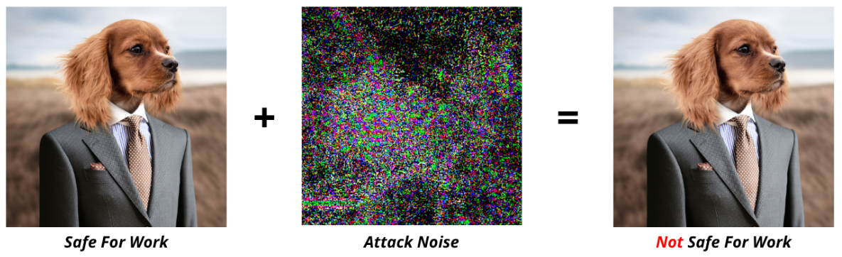
For more details about adversarial examples, an introductory article is now available on this Blog Page from the Skyld website.
In this article, the model used images as input. But what if your model uses something else, like text, audio, or tabular data? Is it still vulnerable?
Is my Model Vulnerable?
With the ART library, a lot of different attacks are available. Each attack can target a specific type of model. This means that many models can fall victim to adversarial examples. The only thing you need to know about this library is that you need to choose the right estimator when selecting the attack and the model, as this is how the link is made between the two.
Here is a table containing all the possible estimators, their input types, and some attacks examples.
| Estimator Type | Domains | Input Types | Typical Attacks |
|---|---|---|---|
| Classifier | Image, Text | Images, Text sequences | FGM, PGD |
| Object Detector | Computer Vision | Images with multiple objects | RobustDPatch |
| Speech Recognizer | Audio Processing | Audio waveforms | ImperceptibleASR |
Before crafting your first adversarial example, let’s see which method we will use.
Projected Gradient Descent
The method used in this article is ProjectedGradientDescent from the ART library. PGD is a white-box attack based on the Fast Gradient Sign Method (FGSM). At each iteration, the method ensures the perturbation is still small i.e. within the allowed perturbation limit according to the chosen norm (l∞ , l1 or l2). You can also customize the following parameters:
-
eps: how much the image can be changed at maximum (e.g. 0.1). -
eps_step: at each step, how much the image is modified. -
max_iter: number of steps for optimization. -
random_init: whether to start with a slightly disturbed image or not
The ProjectedGradientDescent method works with both Object Detection and Image Classification models.
For Image Classification models, the ART library also provides other powerful attack methods, including
Carlini & Wagner,Fast Gradient Sign Method, andAutoProjectedGradientDescent, which can be easily integrated using the same framework.
Customizing for Your Own Model
For this tutorial, we’ll use a YOLOv5s object detector pretrained on the COCO 2017 dataset. You can easily replace the YOLOv5 model with another fine-tuned one by replacing the file chosen in the torch.load(“data/yolov5s.pt”) class UtilsDetectorYolo and updating the COCO_INSTANCE_CATEGORY_NAMES list to reflect the new label set.
To change the model to one other than a YOLOv5, several things need to be redefined:
-
COCO_INSTANCE_CATEGORY_NAMES: Update this list to include the labels and corresponding IDs your new model outputs. -
load_modelupdate this function to:- Provide a wrapper class for your new model:
- Implement a correct
__init__()method and configure the appropriate loss function(s). - Implement the
forward()method to return predictions and compute the loss correctly for both training and inference. The loss must be available to perform adversarial attacks (especially white-box attacks) and can often be guess based on the last model layer.
- Implement a correct
- Save the pretrained model with the desired file.
- Instantiate the appropriate ART estimator, such as PyTorchYolo for YOLO models. Refer to the ART Estimators documentation to choose the correct wrapper class.
- Provide a wrapper class for your new model:
-
load_dataset: Modify this function if you’re using a different data modality (e.g. audio, text). You may also need to change the preprocessing or input transformation steps if your model expects different input dimensions. -
plot_image: Adjust this function if you’re switching to a non-object detection model that uses different visualization logic. -
prediction_format_to_art_format: Convert your model’s raw output format to one compatible with ART’s expected format, depending on your model type and the estimator you use.
Creating an Adversarial Example in Python
Importing Libraries
This is the list of all the major libraries used in the code.
# Standard library imports
import os

# Third-party imports
import cv2
import matplotlib
import matplotlib.pyplot as plt
import numpy as np
import torch
from PIL import Image
from torchvision import transforms

# ART (Adversarial Robustness Toolbox) imports
from art.attacks import EvasionAttack
from art.attacks.evasion import ProjectedGradientDescent
from art.estimators.estimator import BaseEstimator
from art.estimators.object_detection.pytorch_yolo import PyTorchYolo

# YOLO
from yolov5.utils.loss import ComputeLoss

# Local imports
from attacks.white_boxes.local_projected_gradient_descent import LocalProjectedGradientDescent
from attacks.white_boxes.white_box_attack import WhiteBoxAttack
from utils.utils import nms_on_predictions, load_config
from utils.utils_detector_yolo import UtilsDetectorYolo
Configuration
To load a configuration, you need to have your own json file with a correct configuration in it. For this example, the configuration file is data/configs/pgd_default_config.json. If you want to create your own, you have to set all these attributes like in this example:
{
    "THRESHOLD" : 0.6,
    "TARGET_CLASS" : "bird",
    "VICTIM_CLASS" : "airplane",
    "BATCH_SIZE" : 5,
    "IOU_THRESHOLD" : 0.5,
    "MAX_ITER" : 500,
    "NORM" : "inf",
    "EPS" : 1.0,
    "TARGET_LOCATION" : [170, 170],
    "TARGET_SHAPE" : [3, 300, 300],
    "IMAGES_TO_DISPLAY" : 3,
    "FOLDER_NAME" : "original"
}
Then, the file is load in the Notebook like this:
config = load_config("../data/configs/pgd_default_config.json")
Loading a Custom Dataset and a Pre-trained Model
To use the attack, you need a dataset containing the images that will be turned into adversarial examples. This dataset consists of custom images that you must place in the data/custom_images folder. During processing, the images are resized to match the model’s input size (e.g. 640x640). They do not need to be labeled.
Note that the dataset size can be smaller than the batch size if the folder doesn’t contain enough images with the victim class detected. If you encounter this issue, try lowering the threshold used for predictions.
The dataset is loaded immediately after the pre-trained model and can be accessed through the IMAGES variable.
estimated_object_detector = UtilsDetectorYolo(config.BATCH_SIZE, config.THRESHOLD, config.VICTIM_CLASS)
IMAGES = estimated_object_detector.images
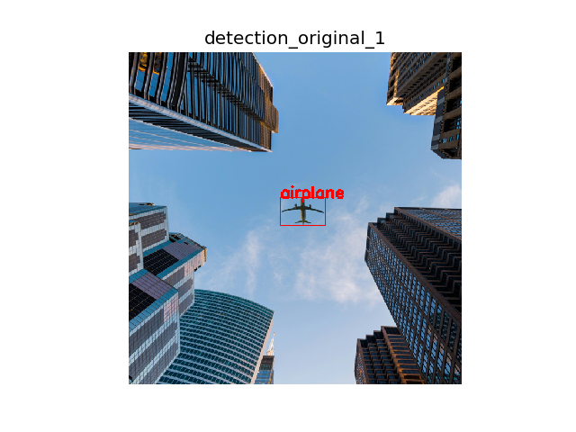
Displaying Predictions of the Dataset
The predict function will add the predictions made by the model on the images from the IMAGES dataset, and save it in the folder data/{FOLDER_NAME}/ with the name detection_{FOLDER_NAME}{_index}.
original_predictions, _ = predict(
        images=IMAGES,
        estimator=estimated_object_detector,
        dataset_name=config.FOLDER_NAME,
        file_name=f"detection_{config.FOLDER_NAME}",
        folder_path=f"../data/{config.FOLDER_NAME}/"
        )
Here is an example image:
Generating the Adversarial Example
You can now generate the adversarial examples from the selected images.
The attack is initialized in the __init__ and generate methods of the LocalProjectedGradientDescent class.
attack = LocalProjectedGradientDescent(
    estimator=estimated_object_detector,
    images=IMAGES,
    orig_predictions=original_predictions,
    target_class=config.TARGET_CLASS
    )

# Generate adversarial examples
_ = attack.generate(
    images = IMAGES,
    orig_predictions = original_predictions,
    target_shape = config.TARGET_SHAPE,
    target_location = config.TARGET_LOCATION,
    norm = config.NORM,
    eps = config.EPS,
    max_iter = config.MAX_ITER
)
Visualizing the Results
Finally, to visualize the attack and generate the adversarial outputs, simply run the apply_attack_to_image method.
# Apply the attack to the images
attack_predictions, adversarial_examples = attack.apply_attack_to_image(
  image=IMAGES,
  train_on=len(IMAGES),
  threshold=config.THRESHOLD,
  )
After generating our adversarial examples and displaying it in the notebook, here is the result obtained:
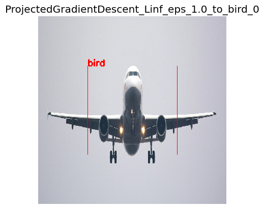
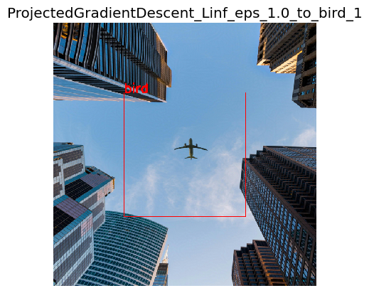
The tested batch contains 5 images featuring airplanes. For the 5 pictures, the YOLOv5s is fooled. The model fails to detect any airplanes and instead predicts only birds.
Now that you’ve seen how to fool an object detector with a few lines of code, what defenses will you put in place?
Defense against Adversarial Examples
Adversarial examples are more and more popular.
But do these attacks only happen in the lab?
As seen in this article, these attacks are really easy to setup, when you have access to the model architecture and its parameters (weights and biases).
So, when an attacker tries to break your AI model, his priority is to obtain the architecture and the parameters. Most of the models in embedded devices are poorly or not protected at all. Defending against adversarial examples before securing the AI model is pointless. It’s like installing antivirus software on a smartphone without setting a password.
For more information about protecting your AI models, please visit Ai-Protection page on the Skyld Website.
Despite everything, if you are still confident about the safety of your models, Skyld can conduct an audit to show you how vulnerable you are. Please visit Skyld’s AdverScan page.